GIFTS TTE Data (gdt.missions.gifts.tte)

Note

The GIFTS TTE data implementation and this document are currently based on those provided by the Fermi Gamma-ray Data Tools, and will be revised in future versions.

TTE (Time-Tagged Event) data is a temporally unbinned time-series of “counts” where each count is mapped to an energy channel. These energy channels are currently a subset of the 128 energy channels provided by a Fermi-GBM GbmTte instance, according to a GIFTS lower energy bound of 20 keV. We can read a TTE file with the GiftsTte class.

>>> from gdt.core import data_path
>>> from gdt.missions.gifts.tte import GiftsTte
>>> tte = GiftsTte.open("gifts/gifts_tte_G3_bn220624124_v00.fit")
>>> tte
<GiftsTte: gifts_tte_G3_bn220624124_v00.fit;
 trigger time: 677732319.512006;
 time range (-131.5836260318756, 474.62935197353363);
 energy range (20.394683837890625, 2000.0)>

Alternatively, the TTE can be retrieved from the current GIFTS burst catalog:

>>> from gdt.missions.gifts.catalogs import BurstCatalog
>>> burstcat = BurstCatalog()
>>> tte = [t for t in burstcat.get_tte(trigger_name="bn220624124") if t.detector=="G3"][0]

The TTE FITS files have multiple data extensions, each with metadata information in a header. There is also a primary header that contains metadata relevant to the overall file. You can access this metadata information:

>>> tte.headers.keys()
['PRIMARY', 'EBOUNDS', 'EVENTS', 'GTI']

Access is provided for certain important properties of the data:

>>> # the good time intervals for the data
>>> tte.gti
<Gti: 1 intervals; range (-131.5853500366211, 474.63367199897766)>

>>> # the trigger time
>>> tte.trigtime
677732319.512006

>>> # the time range
>>> tte.time_range
(-131.5836260318756, 474.62935197353363)

>>> # the energy range
>>> tte.energy_range
(20.394683837890625, 2000.0)

>>> # number of energy channels
>>> tte.num_chans
128

We can retrieve the time-tagged events data contained within the file, which is an EventList class (see Event Data for more details).

>>> tte.data
<EventList: 157347 events;
 time range (-131.5836260318756, 474.62935197353363);
 channel range (16, 127)>

The PhotonList base class provides a number of high-level functions, such as slicing the data in time:

>>> time_sliced_tte = tte.slice_time((-10.0, 10.0))
>>> time_sliced_tte
<GiftsTte:
 trigger time: 677732319.512006;
 time range (-9.999047994613647, 9.999963998794556);
 energy range (20.394683837890625, 2000.0)>

As TTE data is temporally unbinned, it must be initially binned in time prior to the generation of a lightcurve, where the Binning Algorithms for Unbinned Data can be used. For this example, bin_by_time() bins the TTE to the specified time resolution, converting the TTE to a PHAII object:

>>> from gdt.core.binning.unbinned import bin_by_time
>>> phaii = tte.to_phaii(bin_by_time, 1.024, time_ref=0.0)
>>> phaii
<GiftsPhaii:
 trigger time: 677732319.512006;
 time range (-132.096, 475.136);
 energy range (4.062646865844727, 2000.0)>

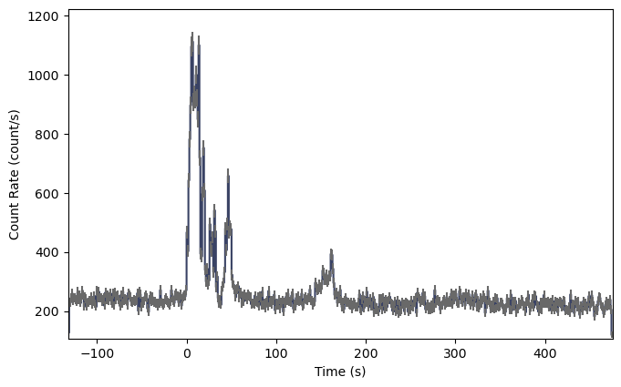
Here, we binned the data to 1.024 s resolution, where the reference point at which to start the binning (in both directions) was at T0=0 s. The resulting GiftsPhaii object can be used to generate a lightcurve using the Lightcurve class:

>>> import matplotlib.pyplot as plt
>>> from gdt.core.plot.lightcurve import Lightcurve
>>> lcplot = Lightcurve(data=phaii.to_lightcurve())
>>> plt.show()

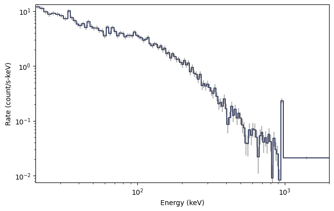
To plot the spectrum, no additional binning is required as the TTE is already necessarily pre-binned in energy. A spectrum plot can be generated directly from the TTE object without any extra steps using the Spectrum class:

>>> from gdt.core.plot.spectrum import Spectrum
>>> # integrate over time from 0 - 10 s
>>> spectrum = tte.to_spectrum(time_range=(0.0, 10.0))
>>> specplot = Spectrum(data=spectrum)
>>> specplot.xlim = tte.energy_range
>>> plt.show()

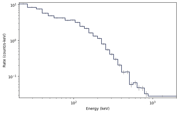
If required, the count spectrum can be rebinned using one of the Binning Algorithms for Binned Data. For example, combine_by_factor() combines bins together by an integer factor:

>>> from gdt.core.binning.binned import combine_by_factor
>>> # rebin the count spectrum by a factor of 4
>>> rebinned_energy = tte.rebin_energy(combine_by_factor, 4)
>>> rebinned_spectrum = rebinned_energy.to_spectrum(time_range=(0.0, 10.0))
>>> specplot = Spectrum(data=rebinned_spectrum)
>>> specplot.xlim = tte.energy_range
>>> plt.show()

See Plotting Lightcurves and Plotting Count Spectra for more on how to modify these plots.

Finally, we can write out a new fully-qualified GIFTS TTE FITS file after some reduction tasks. For example, we can write out our time-sliced data object:

>>> time_sliced_tte.write('./', filename='my_first_custom_tte.fit')

For more details about working with TTE data, see Photon List and Time-Tagged Event Files.

Reference/API

gdt.missions.gifts.tte Module

Classes

GiftsTte()

Class for Time-Tagged Event data.

Class Inheritance Diagram